Machine-learning-based approaches have been utilized to effectively categorize lung tumors with various mutational statuses, as well as gastrointestinal cancers depending on microsatellite instability conditions.
There is growing interest in using neural networks to grade prostate cancer (PCa), and several recent studies have touched on the possibility of using deep learning (DL) algorithms to predict PCa progression and survival. Artificial intelligence (AI), or more accurately trained neural networks, has shown considerable potential in recognizing histological morphologies and changes previously identified by pathologists.
After primary therapy for PCa, Gleason grading is the best predictor of survival. Gleason grade patterns have been adjusted and recapitulated into GS 6 to 10 since the establishment of the Gleason Score (GS) in 1966.
Since it is easier and more accurately represents the PCa result, a new method with five separate grade groups (GGs) has been adopted to be used in combination with the Gleason grading. Furthermore, because GGs are dependent on altered GS groups, Gleason’s grading accuracy is just as critical as before (Table 1).
Table 1. Grade grouping based upon Gleason scores. Source: Sandeman, et al., 2022
| ISUP Grade Group |
Gleason Score |
| GG1 |
3 + 3 |
| GG2 |
3 + 4 |
| GG3 |
4 + 3 |
| GG4 |
4 + 4, 3 + 5, 5 + 3 |
| GG5 |
4 + 5, 5 + 4, 5 + 5 |
ISUP = International Society of Urological Pathology.
AI approach has lately questioned PCa-related intra- and interobserver inconsistency. In particular, neural networks have mainly been achieved in the binomial categorization of benign tissue vs. cancer or in grading prostate samples to the level of professional pathologists. Any neural-network-based method must therefore excel in outcome prediction to be useful in everyday pathology practice and decision making.
Researchers used a comparatively small training sample to construct a strong Gleason grade classifier in prostate biopsies. For the diagnosis of cancer recurrence following initial treatment, researchers set out to develop a precise and effective algorithm that also reproduces the features of grading.
Methodology
Between 2016 and 2017, researchers studied 750 patients who had a prostate biopsy at the Helsinki University Hospital (HUS). Table 2 shows the demographics of the cohort.
Table 2. Characteristics of the men diagnosed with prostate cancer and the subcohort that underwent surgical treatment. Source: Sandeman, et al., 2022
| Full Cohort |
|
n, Mean, or Median |
Percentage, SD, or IQR |
| Patients, n |
|
750 |
100 |
| Age (years), mean (SD) |
|
68.1 |
8.09 |
| Biopsies, n |
|
871 |
100 |
| Biopsy series, n (%) |
1 |
653 |
87.07 |
| 2 |
84 |
11.2 |
| 3 |
3 |
0.4 |
| 4 |
9 |
1.2 |
| 5 |
0 |
0 |
| 6 |
1 |
0.13 |
| Biopsy ISUP grade group, n (%) |
0 |
258 |
34.4 |
| 1 |
113 |
15.07 |
| 2 |
169 |
22.53 |
| 3 |
114 |
15.2 |
| 4 |
28 |
3.73 |
| 5 |
68 |
9.07 |
| PSA (ng/L), median (IQR) |
|
8.5 |
4.5 |
| RALP Cohort |
|
n, Mean, or Median |
Percentage, SD, or IQR |
| Patients, n (%) |
|
126 |
100 |
| Biopsies, n (%) |
|
146 |
100 |
| Age at RALP (years), mean (SD) |
|
64.8 |
7.1 |
| Biopsy series, n (%) |
1 |
106 |
84 |
| 2 |
20 |
16 |
| Biopsy ISUP grade group, n (%) |
0 |
0 |
0 |
| 1 |
14 |
11 |
| 2 |
56 |
44.44 |
| 3 |
42 |
33 |
| 4 |
7 |
6 |
| 5 |
7 |
6 |
| Preoperative PSA (ng/L), median (IQR) |
|
8.5 |
4.5 |
| Prostatectomy pT, n (%) |
2 |
70 |
56 |
| 3a |
37 |
29 |
| 3b |
19 |
15 |
| pN, n (%) |
0 |
110 |
87 |
| 1 |
16 |
13 |
| BCR relapse PSA (ng/L), median (IQR) (n = 19) |
|
0.59 |
1.07 |
| Months to BCR relapse, median (IQR) |
|
10.58 |
27.71 |
ISUP = International Society of Urological Pathology; PSA = prostate-specific antigen; RALP = robot-assisted radical prostatectomy; BCR = biochemical recurrence; pT = primary tumor pathological stage; pN = lymph node stage.
A set of 872 biopsy sessions yielded 4221 hematoxylin-and-eosin-stained (H&E) slides for AI development (Figure 1).
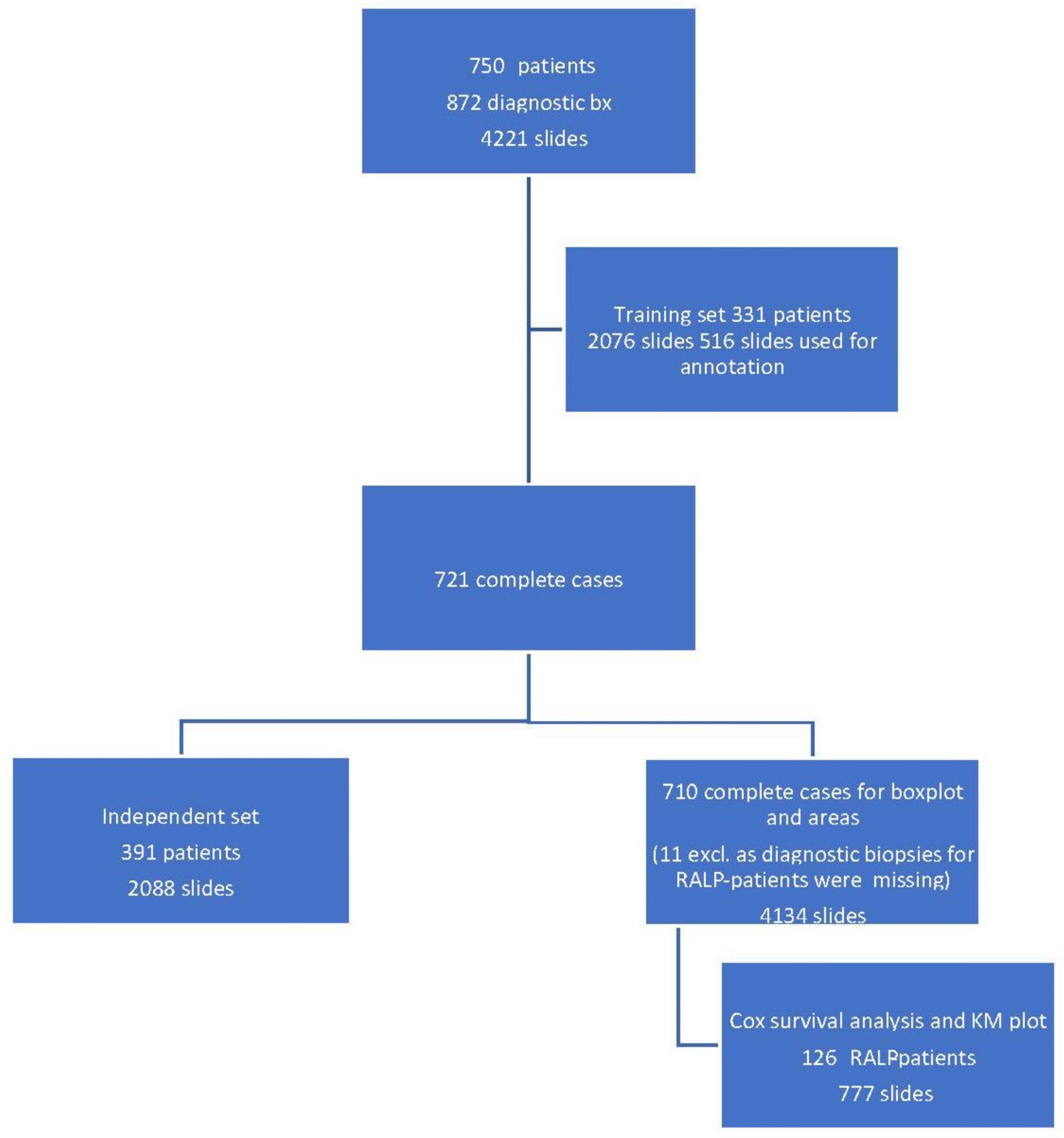
Figure 1. Workflow of the study cohort data selection depicting a training set, an independent set, and a radical prostatectomy (RALP) patient cohort from 872 prostate core biopsy series. Image Credit: Sandeman, et al., 2022
All of the patients’ clinical and pathological information was gathered. The extraprostatic extension (EPE), seminal vesicle invasion (SVI), node status (NS), and pathologic stage (pT) data for RALP patients were obtained from computerized surgical pathology records.
EPE, SVI, or positive NS were characterized as negative pathologic findings in RALP specimens. For survival data, all postoperative prostate-specific antigen (PSA) results were calculated during the follow-up period.
Two independent convolutional neural networks (CNNs) for multi-class semantic segmentation of tissue (CNN-T) and Gleason grades (CNN-GG) were developed for the AI algorithm. The training was completely supervised, and the training data was labeled as powerful pixel-level multi-class segments in the Aiforia software by two experienced uropathologists in agreement for both tissue and Gleason grades.
To boost the effectiveness of the AI algorithm, iterations were used to train the system. Primary annotations, annotation corrections, and the inclusion of new portions from independent material were all part of the training, which was reliant on outliers in the AI vs. pathologist confusion matrix.
The optimal minimum for the filter area, which coincided with benign vs. malignant classification and also GG stratification, was then found using an area filter curve depending on this confusion matrix (Figure 2).
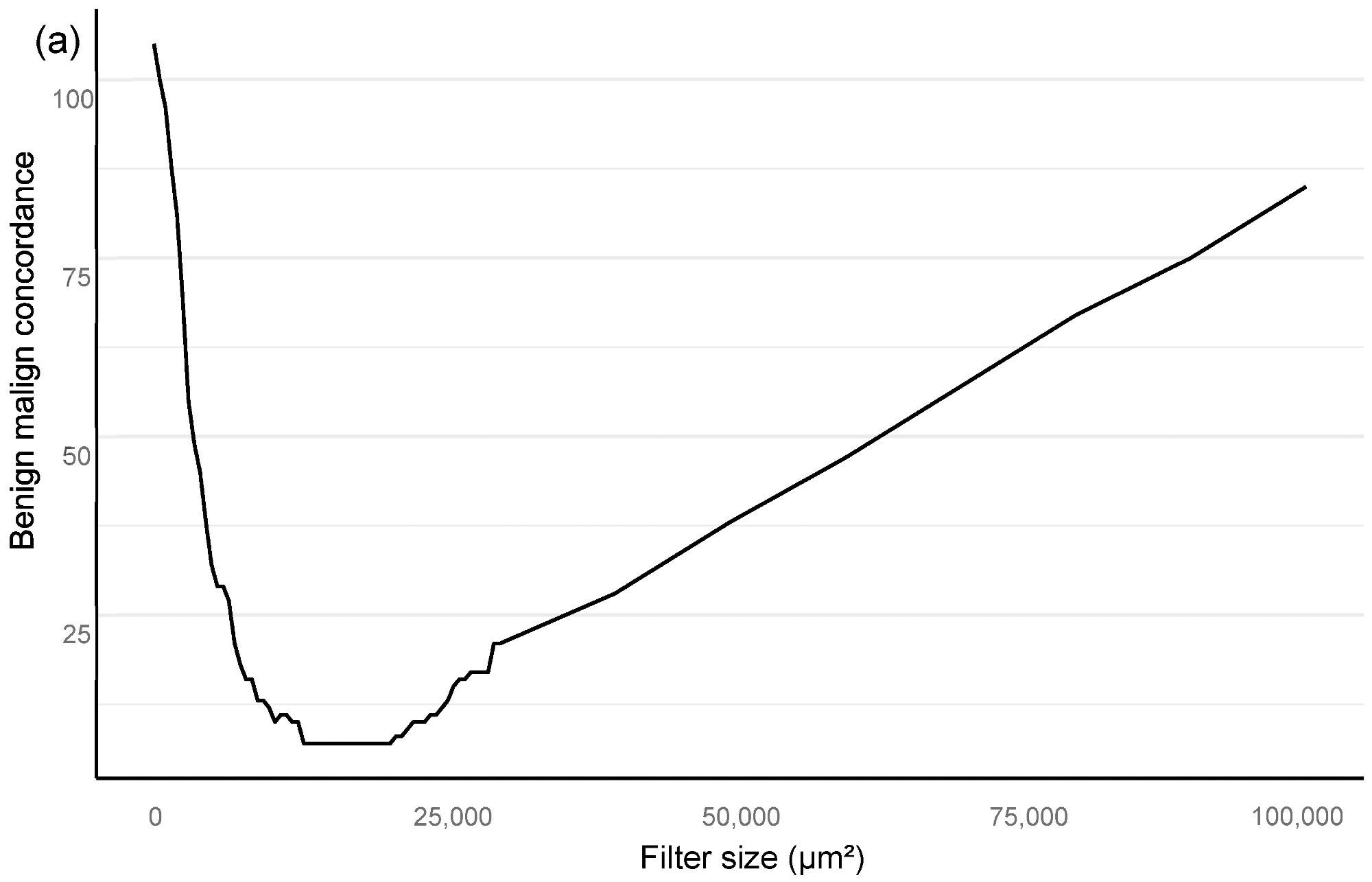
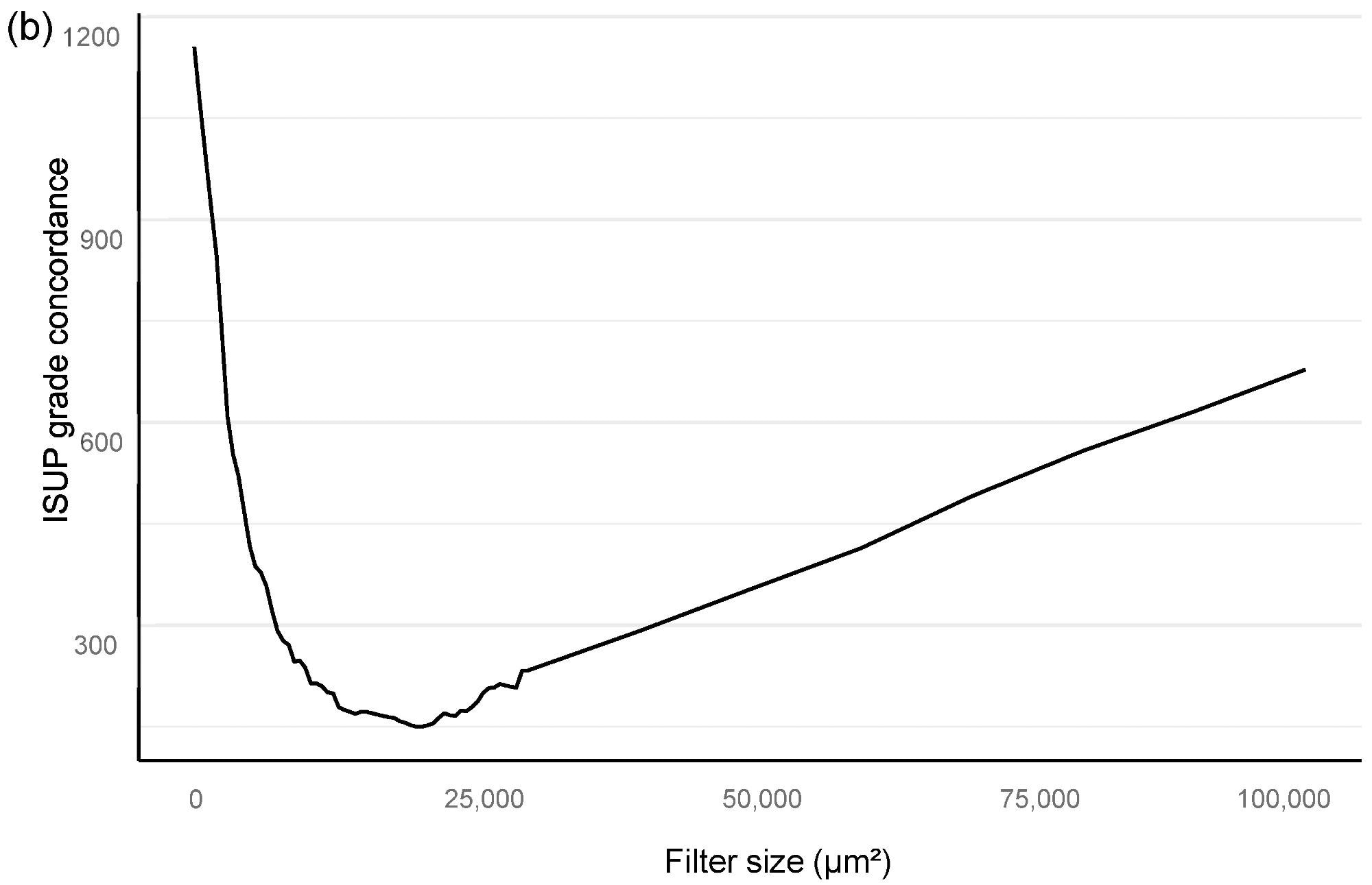
Figure 2. Bloom filter for the determination of the minimal filter size for benign versus malign tissue (a) and grade group difference (b) based upon the clinical performance of the algorithm compared to clinical diagnosis. Image Credit: Sandeman, et al., 2022
The filter curve was created by a clinical process. The AI system training material was a subset of 516 slides chosen from a total of 2076 slides submitted by 331 patients. On the training set slides, a total of 3606 glandular regions and stromal backdrops were annotated, yielding a total area of 94 mm2 of fully annotated prostate tissue (Table 3).
Table 3. Total area per annotated class in the training set of 516 biopsy slides. Source: Sandeman, et al., 2022
| Class |
Total Area in mm2 |
| Benign |
58.24 |
| G3 |
9.41 |
| G4 |
10.27 |
| G4 cribriform |
6.28 |
| G5 |
9.7 |
Results and Discussion
Researchers mathematically predicted a minimum region for histological class classification that would not overlook a clinically important malignancy because the approach to obtaining the optimum deep neural network solution is reliant on pixel-level annotations and whole biopsy session (patient-level) ground truth for a GG.
Based on an analysis of the AI model’s sensitivity and specificity to the pathology report, the Bloom filter curve approach revealed the appropriate filter size for benign vs. malignant and GG categorization (Figure 2).
Our algorithm’s ideal filter area was 15,000 square μm (Figure 2), leading to an AUC of 0.997 in ROC AUC evaluation for identifying malignant vs. benign (Figure 3).
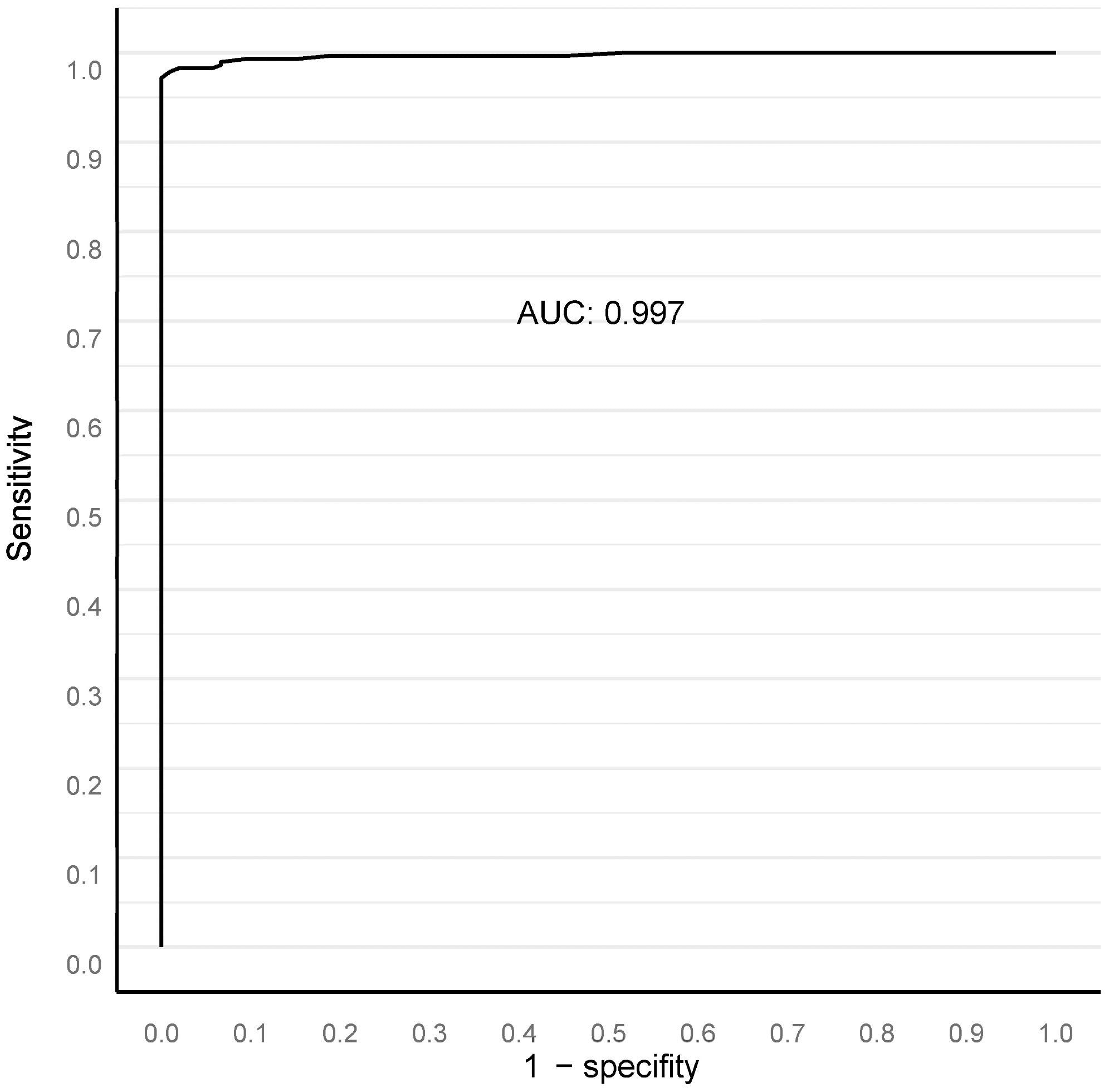
Figure 3. ROC AUC analysis for benign versus malignant compared to clinical diagnosis at the full biopsy session level, with a 15,000 square micron filter applied (see text). Image Credit: Sandeman, et al., 2022
Even from a clinical standpoint, the filter still includes small tumor regions that a uropathologist would recognize in a biopsy series, as shown in Figure 4.
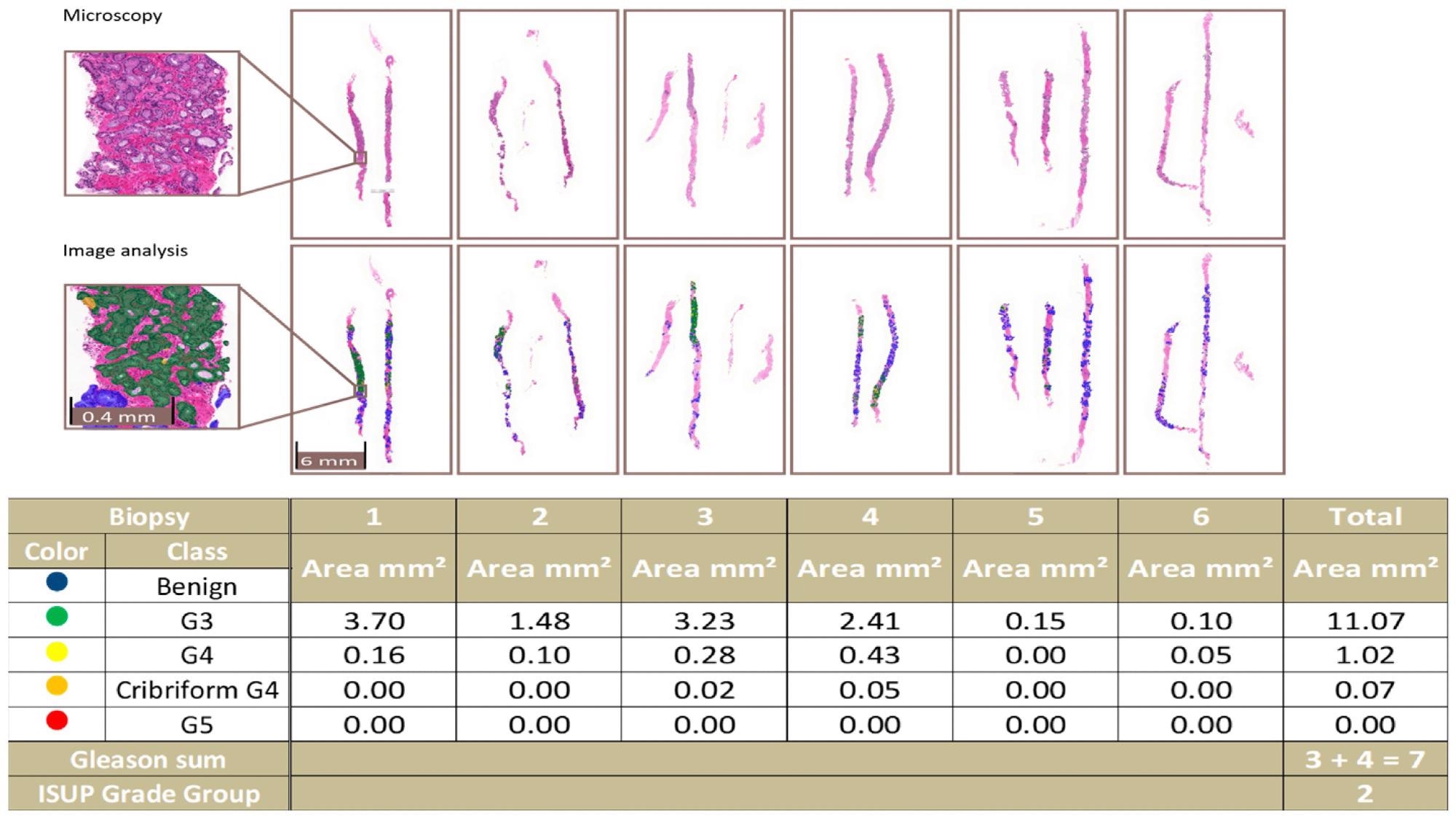
Figure 4. An example of a complete biopsy session slide set. Image analysis data are produced by pixel-level multi-class semantic segmentation at the level of the individual biopsy slide and compiled at the level of the complete slide set. In the example, the patient-level ISUP grade group is 2. Image Credit: Sandeman, et al., 2022
In a confusion matrix, researchers compared the results of AI and the pathologist at the original diagnosis to optimize the algorithm. Five false negatives (1%) and two false positives were detected by AI. In 111 cases (24%), there was a disagreement between AI and the pathologists due to one GG in PCa (Table 4).
Table 4. Confusion matrix for the grade group in complete biopsy sessions by the pathologist versus AI. Distribution of patient-level grade groups (A). Percentage distribution (B). Source: Sandeman, et al., 2022
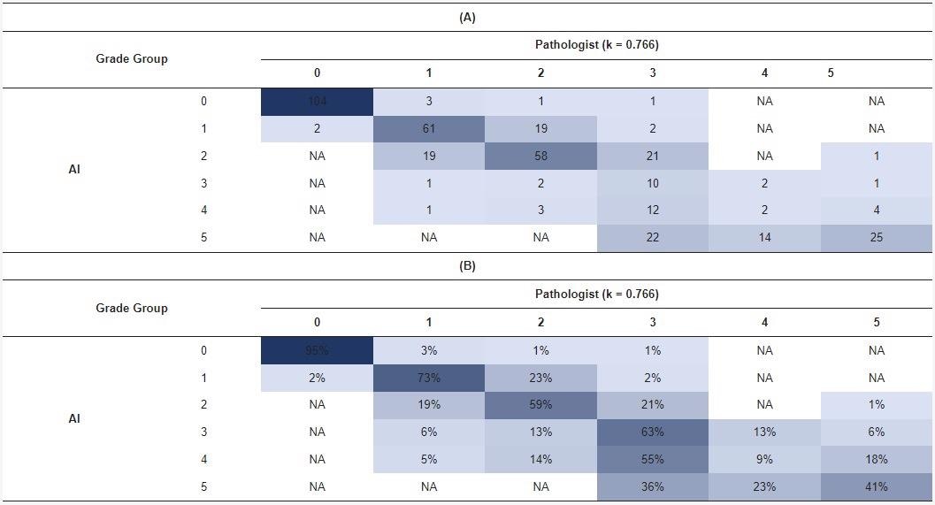
The blue shading represents the number (A) or percentage (B) of cases in each cell of the matrix.
For the benign class, including each GG, sensitivity, specificity, negative predictive value (NPV), and positive predictive value (PPV) were computed (Table 5).
Table 5. Accuracy of the AI algorithm: Predictive values for all classes. Source: Sandeman, et al., 2022
| |
Class |
| Benign |
GG1 |
GG2 |
GG3 |
GG4 |
GG5 |
| Cases, n (%) |
112 (28%) |
85 (21%) |
83 (21%) |
68 (17%) |
18 (5%) |
31 (8%) |
| Sensitivity |
0.98 |
0.72 |
0.70 |
0.15 |
0.11 |
0.81 |
| Specificity |
0.98 |
0.93 |
0.87 |
0.98 |
0.95 |
0.90 |
| PPV |
0.96 |
0.73 |
0.59 |
0.63 |
0.09 |
0.41 |
| NPV |
0.99 |
0.92 |
0.92 |
0.85 |
0.96 |
0.98 |
Accuracy = 0.67. Cohen’s weighted kappa = 0.77. p < 0.0001
The technique yielded an overall weighted kappa value of 0.76 (p < 0.0001). For clinically meaningful cohorts ISUP GG1−2 versus ISUP GG3 to 5, predictive values for algorithm efficiency were obtained (Table 6).
Table 6. Accuracy of the AI algorithm: Predictive values for dichotomized groups. Source: Sandeman, et al., 2022
| Class |
| |
Benign versus Malign |
Benign to Grade 1 versus 2–5 |
Benign to Grade 2 versus 3–5 |
Only Malignant Cases Grade 1 versus 2–5 |
Only Malignant Cases Grade 1–2 versus 3–5 |
| Number of Cases |
112/285 |
197/200 |
280/117 |
85/200 |
168/117 |
| Sensitivity |
0.98 |
0.89 |
0.98 |
0.75 |
0.96 |
| Specificity |
0.98 |
0.89 |
0.79 |
0.89 |
0.79 |
| PPV |
0.96 |
0.88 |
0.92 |
0.74 |
0.87 |
| NPV |
0.99 |
0.89 |
0.93 |
0.89 |
0.93 |
| Accuracy |
0.98 |
0.89 |
0.92 |
0.85 |
0.89 |
| Cohen’s Kappa (p < 0.0001) |
0.96 |
0.78 |
0.80 |
0.63 |
0.76 |
The overall area and percentage of cancer discovered by AI per biopsy session were plotted against the pathologist’s identification of GGs, revealing a logical shift in AI-diagnosed grade patterns that corresponded to the pathologist’s diagnoses (Figure 5).
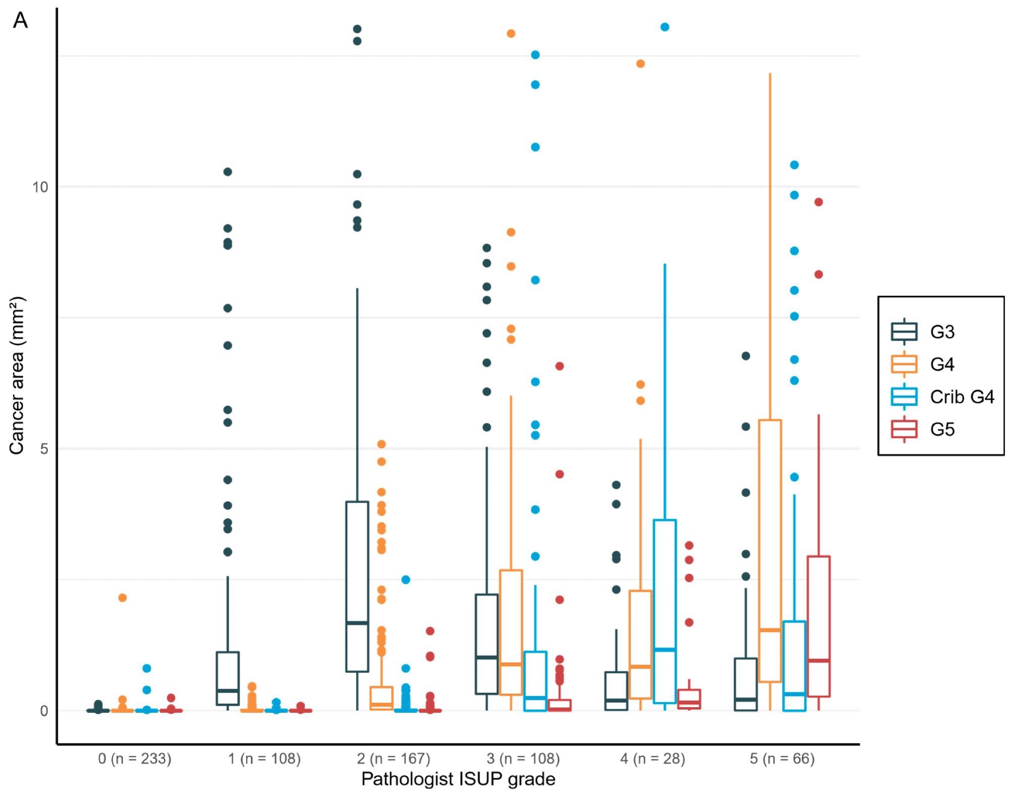
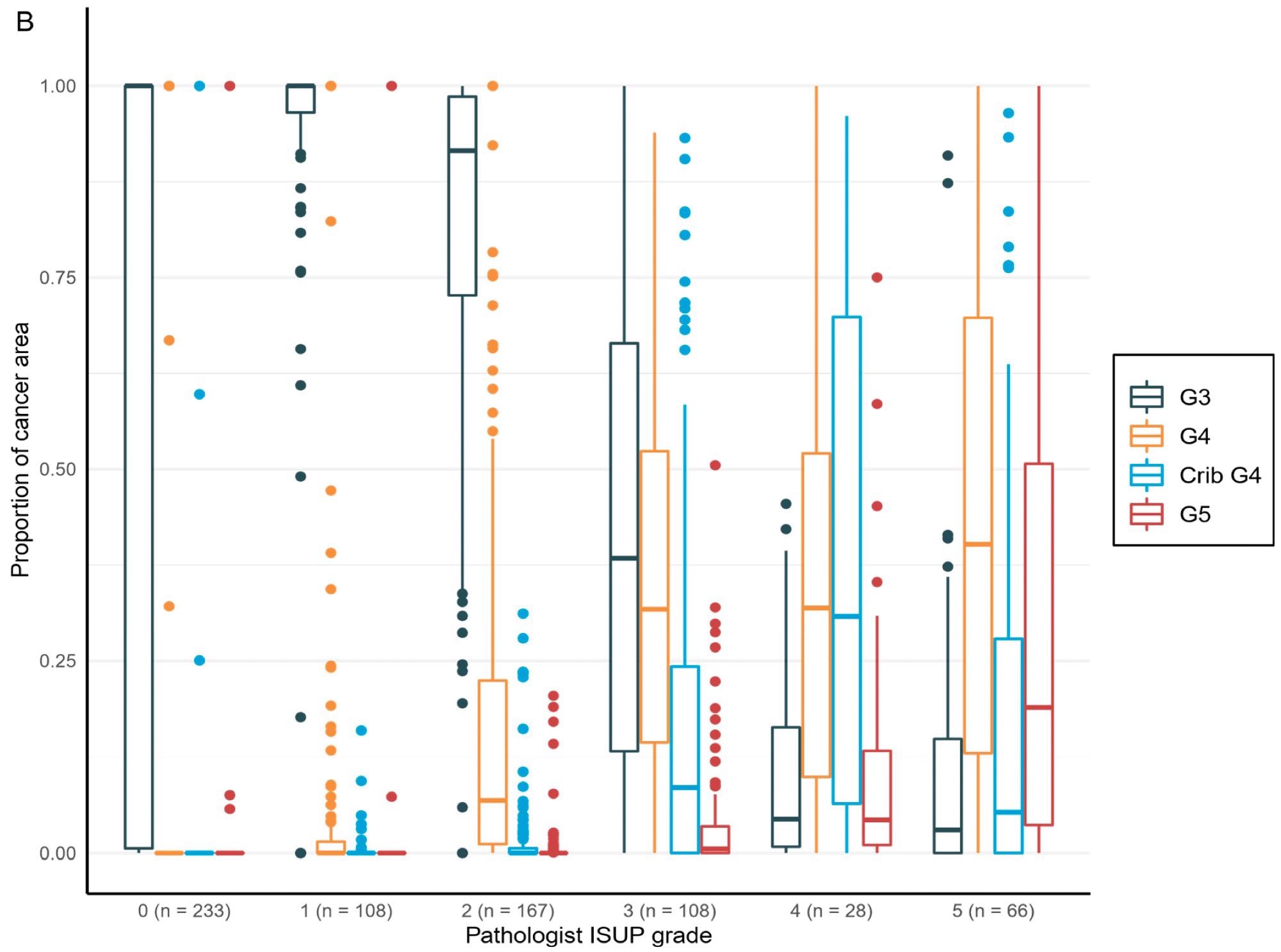
Figure 5. Distribution of the Gleason grade in the area (A) and percentage of the cancer area (B) by AI compared to the grade group by the pathologist. Total n = 710. Image Credit: Sandeman, et al., 2022
Logistic regression models added statistically meaningful connections between the tumor area evaluated by AI for all classes and the pathologists’ clinical diagnosis to the proportions presented in the boxplots (Table 7).
Table 7. Generalized linear modeling demonstrates a statistically significant relationship between the clinical GG and the AI-determined tumor area for each class for the independent set, indicating that every AI-determined-class-dependent tumor area attributes to the AI-assessed GG in a similar way as the pathologist. Source: Sandeman, et al., 2022
| Tumor Area in mm2 |
Odds Ratio |
95% CI |
p |
| G3 |
1.14 |
(1.08–1.19) |
<0.0001 * |
| G4 |
1.14 |
(1.1–1.18) |
<0.0001 * |
| Cribriform G4 |
1.22 |
(1.16–1.28) |
<0.0001 * |
| G5 |
1.08 |
(1.05–1.12) |
<0.0001 * |
n = 397; *: p-values < 0.05 were considered significant.
In both the AI-determined biopsy GG and the human-observer-determined biopsy GG, AI comparisons between the biopsy session GG and the RALP GG were downgraded and upgraded. The deviation from the midpoint was observed to be higher in the AI-graded biopsy than in the original biopsy in the confusion matrixes (Table 8).
Furthermore, the observed tertiary grade pattern in RALP was connected with the increased number of GG5 in AI-determined biopsy grades contrasted to pathologists’ GG5 (Table 8).
Table 8. Cross tabulation showing down- and upgrading of the biopsy session GG in the RALP specimen. Source: Sandeman, et al., 2022
| RALP GG |
| AI biopsy GG |
0 |
1 |
2 |
3 |
4 |
5 |
| 0 |
0 |
0 |
0 |
0 |
1 |
0 |
| 1 |
0 |
0 |
10 |
3 |
0 |
0 |
| 2 |
0 |
0 |
40 |
23 |
0 |
0 |
| 3 |
0 |
0 |
3 |
5 |
0 |
0 |
| 4 |
0 |
0 |
4 |
9 |
2 |
0 |
| 5 |
0 |
0 |
0 |
16 |
2 |
8 |
| RALP GG |
| Pathologist biopsy GG |
0 |
1 |
2 |
3 |
4 |
5 |
| 0 |
0 |
0 |
0 |
0 |
0 |
0 |
| 1 |
0 |
0 |
11 |
3 |
0 |
0 |
| 2 |
0 |
0 |
42 |
13 |
1 |
0 |
| 3 |
0 |
0 |
3 |
36 |
2 |
1 |
| 4 |
0 |
0 |
0 |
4 |
0 |
3 |
| 5 |
0 |
0 |
1 |
0 |
2 |
4 |
For the overall area, the value of AI in predicting unfavorable cancer extent after surgery was examined. Furthermore, the percentage of malignancy discovered by AI during each biopsy session was compared to the negative pathology results of prostatectomy (Figure 6).
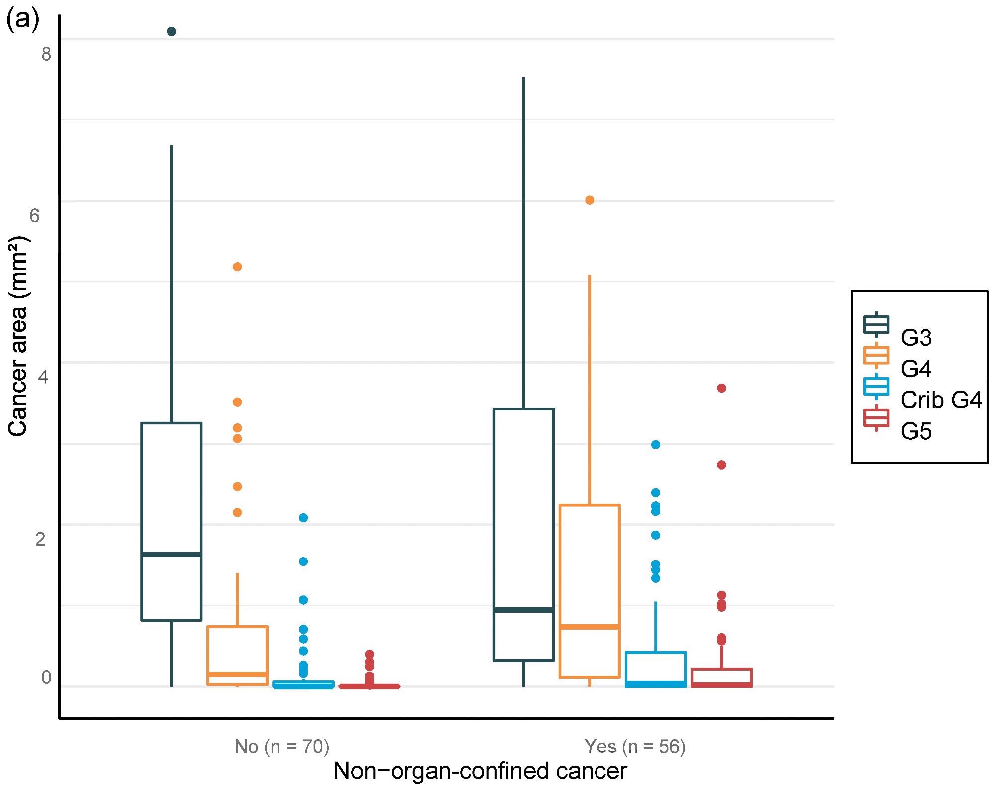
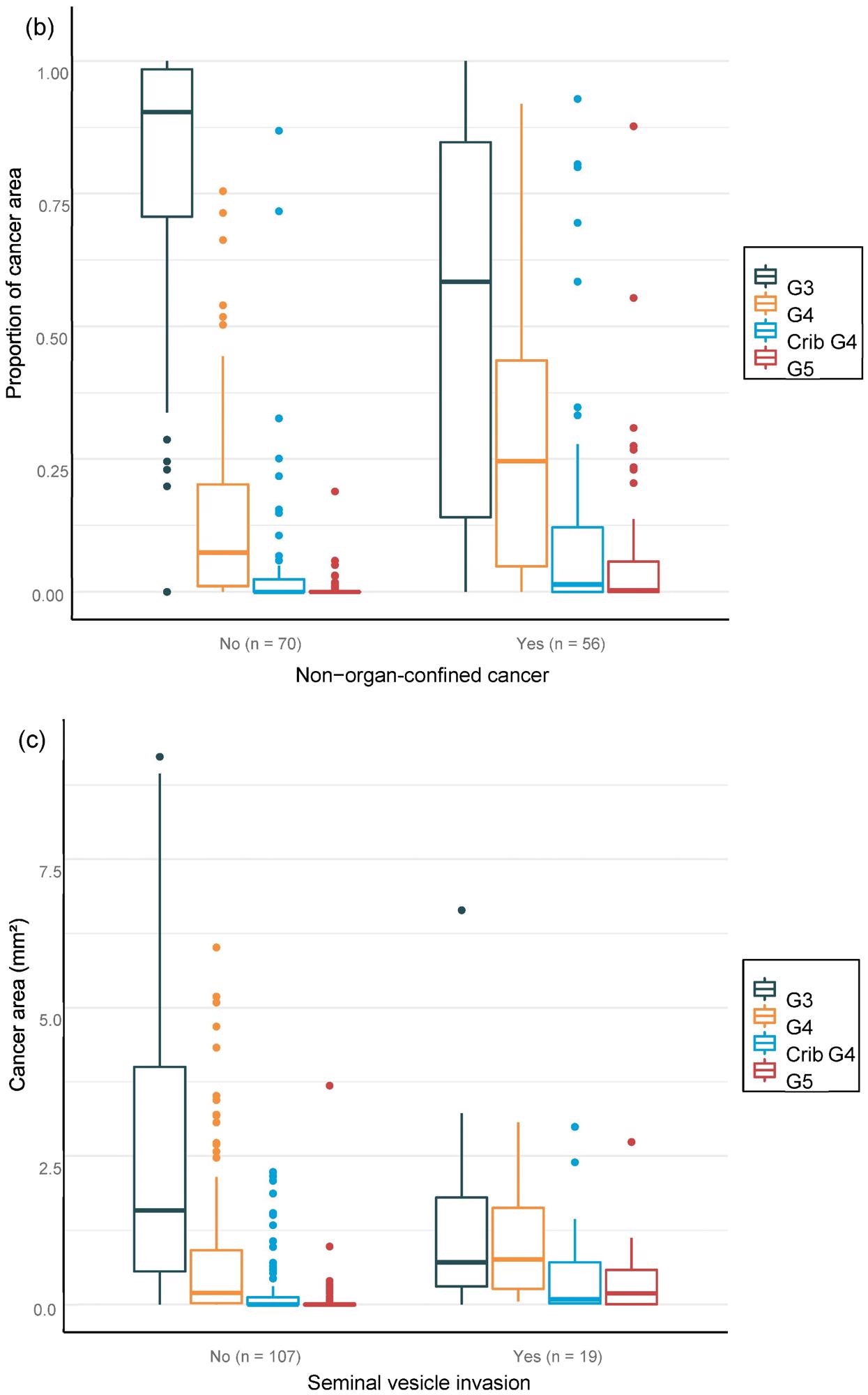
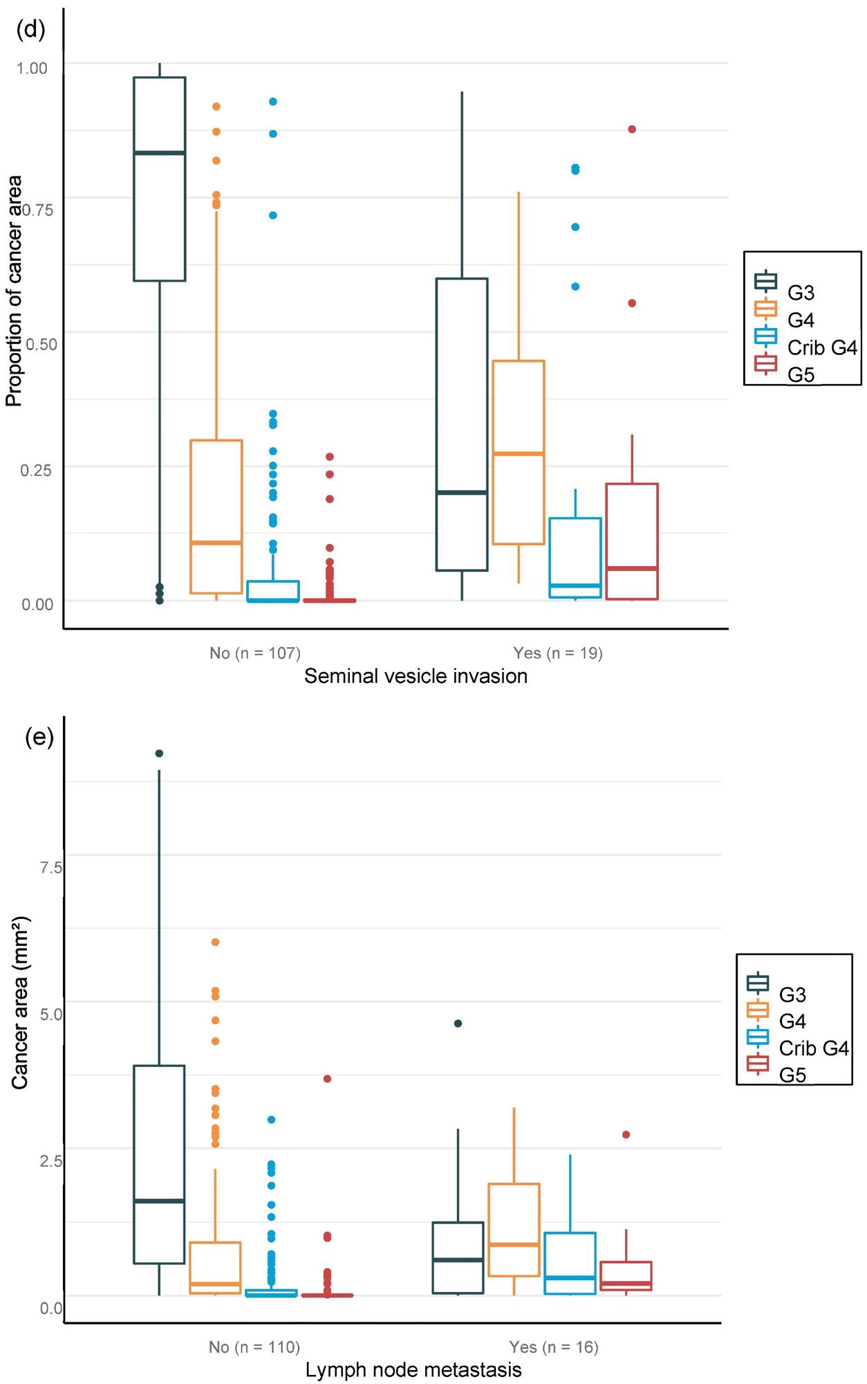
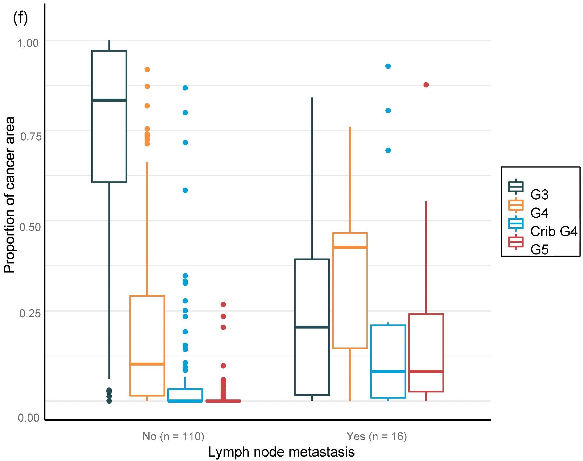
Figure 6. Distribution of Gleason grade in the area (a,c,e) and percentage of cancer area (b,d,f) by AI on biopsy session compared to adverse events non-organ confined (a,b), seminal vesicle invasion (c,d), and lymph node involvement (e,f) at prostatectomy. Image Credit: Sandeman, et al., 2022
Multiple logistic regression studies of the grade pattern 5 area, in particular, demonstrated a statistically significant link to negative pathology results. SVI and LN metastasis at RALP were substantially linked with AI-assigned regions of cribriform grade 4 and grade 5 in biopsies (Table 9).
Table 9. Multi-regression models for adverse pathological findings at prostatectomy show a statistically significant correlation between the area of cribriform G4 and G5 for seminal vesicle invasion and lymph node metastasis, as G5 shows high OR for non-organ-confined disease. Source: Sandeman, et al., 2022
| Clinical Outcome |
Tumor Area in mm2 |
Odds Ratio |
95% CI |
p |
| Non-organ-confined disease |
G3 |
0.93 |
(0.78–1.07) |
0.35 |
| G4 |
1.39 |
(0.99–2.04) |
0.07 |
| Cribriform G4 |
1.89 |
(0.89–4.70) |
0.12 |
| G5 |
48.52 |
(3.03–4125) |
0.03 * |
| Seminal vesicle invasion |
G3 |
0.82 |
(0.56–1.07) |
0.22 |
| G4 |
0.72 |
(0.41–1.10) |
0.17 |
| Cribriform G4 |
2.46 |
(1.16–5.45) |
0.02 * |
| G5 |
5.58 |
(1.57–30.56) |
0.02 * |
| Lymph node metastasis |
G3 |
0.73 |
(0.44–1.03) |
0.13 |
| G4 |
0.8 |
(0.48–1.20) |
0.32 |
| Cribriform G4 |
2.66 |
(1.23–6.06) |
0.01 * |
| G5 |
4.09 |
(1.25–20.12) |
0.04 * |
*: p-values < 0.05 were considered significant
The GG assessed by pathologists or AI strongly classified the patients with a distinct probability for BCR following RALP, according to a Kaplan–Meier survival evaluation. This was also accurate after stratifying patients into GG1–2 and GG3–5 groups, where the survival curves were more clearly separated for the neural-network-based GG evaluation (Figure 7).
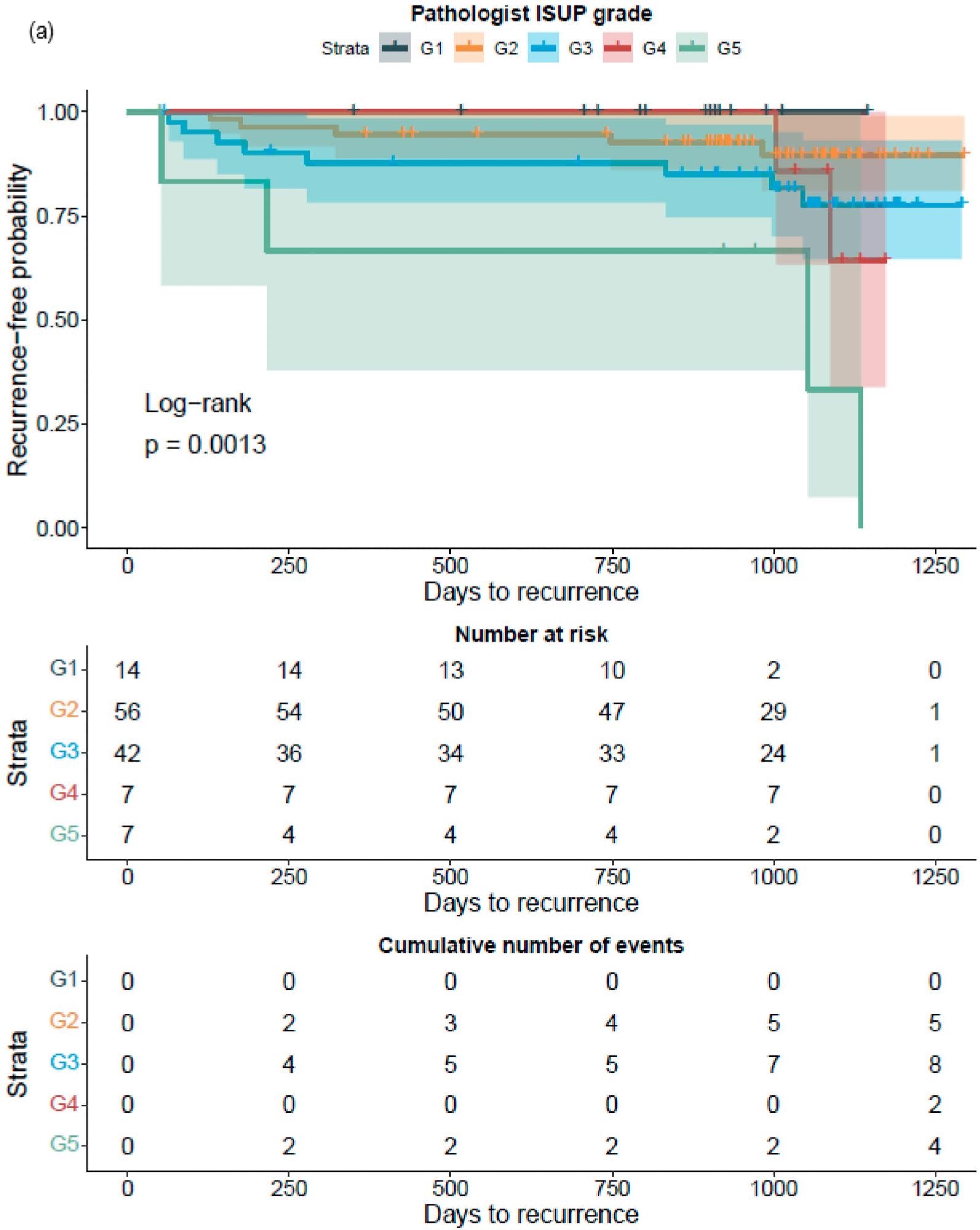
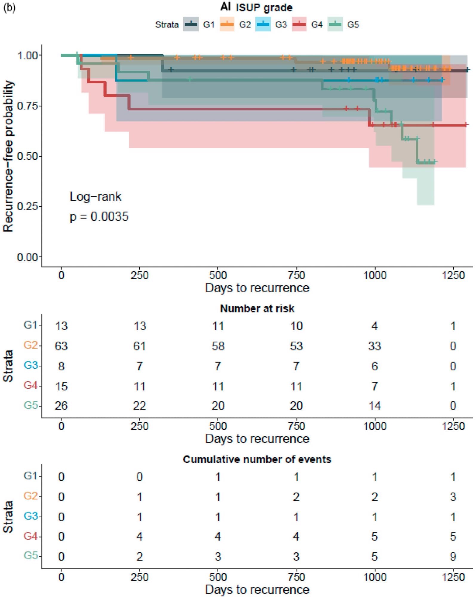
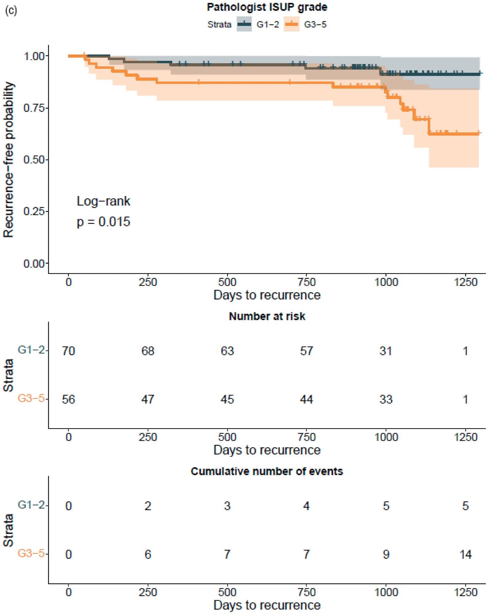
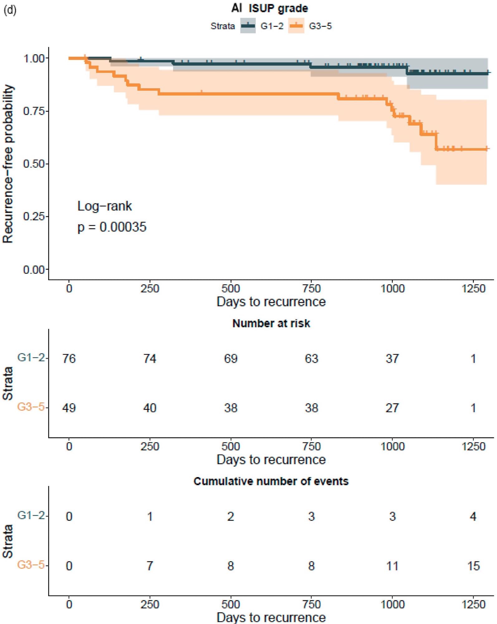
Figure 7. Kaplan–Meier survival analysis for biochemical recurrence on non-stratified (a,b) and stratified (1–2 versus 3–5) (c,d) cancer-positive biopsies for the prostatectomy cohort. The graph shows 95% confidence intervals. Image Credit: Sandeman, et al., 2022
An increase in the GG was similarly related to a higher probability of BCR, regardless of the observer, i.e. pathologist or AI, according to a Cox proportional HR analysis for BCR (Table 10).
Table 10. Cox proportional-hazard regression analysis. Source: Sandeman, et al., 2022
| Parameter |
Hazard Ratio |
95% CI |
p |
| Pathologist ISUP GG |
2.09 |
(1.38–3.16) |
<0.001 * |
| AI ISUP GG |
1.80 |
(1.27–2.53) |
<0.001 * |
| AI Gleason |
2.15 |
(1.34–3.44) |
<0.01 * |
| G3 area (mm2) |
0.94 |
(0.77–1.14) |
0.51 |
| G4 area (mm2) |
1.03 |
(0.99–1.06) |
0.19 |
| Crib G4 area (mm2) |
1.13 |
(0.57–2.24) |
0.72 |
| Total G4 area (mm2) |
1.03 |
(0.99–1.07) |
0.18 |
| G5 area (mm2) |
1.10 |
(0.99–1.23) |
0.07 |
| Total cancer area (mm2) |
1.02 |
(0.99–1.05) |
0.22 |
| G3 proportion of cancer (%) |
0.13 |
(0.04–0.47) |
<0.01 * |
| G4 proportion of cancer (%) |
3.59 |
(0.65–19.72) |
0.14 |
| Crib G4 proportion of cancer (%) |
2.94 |
(0.52–16.59) |
0.22 |
| Total G4 proportion of cancer (%) |
3.97 |
(0.99–15.9) |
0.05 |
| G5 proportion of cancer (%) |
243.7 |
(28.8–2062) |
<0.001 * |
| Strata |
| Pathologist ISUP GG1–2 versus 3–5 |
3.31 |
(1.19–9.23) |
0.02 * |
| AI ISUP GG1–2 versus 3–5 |
5.91 |
(1.96–17.83) |
<0.01 * |
n = 126; *: p-values < 0.05 were considered significant.
Researchers were able to verify that the AI-based region of cribriform G4 and G5 in prostate biopsies was linked to RALP negative outcomes, including seminal vesicle invasion and positive lymph node condition. The region of G5 in biopsies was found to be substantially linked to non-organ-confined illness. The fraction of GG pattern 5 is a major predictor of BCR, according to the findings.
Finally, histology may reveal physiologically and therapeutically relevant signals that the human eye misses, thus improving our capacity to forecast cancer behavior. Within a particular GG, AI-based approaches may assist in stratifying patients with varying lifespans. Shared decision-making combined with supportive multidisciplinary prognostics models is likely to be the future of medical decision-making.
Conclusion
This study demonstrates that AI can detect and grade PCa in biopsies in a manner comparable to pathologists. In a prostatectomy specimen, AI anticipates unfavorable staging and the likelihood of post-operative BCR as well as a pathologist.
Journal Reference:
Sandeman, K., Blom, S., Koponen, V., Manninen, A., Juhila, J., Rannikko, A., Ropponen, T., Mirtti, T. (2022) AI Model for Prostate Biopsies Predicts Cancer Survival. Diagnostics, 12(5), p. 1031. Available Online: https://www.mdpi.com/2075-4418/12/5/1031/htm.
References and Further Reading
- Mukhopadhyay, S., et al. (2018) Whole Slide Imaging versus Microscopy for Primary Diagnosis in Surgical Pathology: A Multicenter Blinded Randomized Noninferiority Study of 1992 Cases (pivotal Study). The American Journal of Surgical Pathology, 42, pp. 39–52. doi.org/10.1097/PAS.0000000000000948.
- Mills, A. M., et al. (2018) Diagnostic Efficiency in Digital Pathology: A Comparison of Optical versus Digital Assessment in 510 Surgical Pathology Cases. The American Journal of Surgical Pathology, 42, pp. 53–59. doi.org/10.1097/PAS.0000000000000930.
- Stålhammar, G., et al. (2018) Digital Image Analysis of Ki67 in Hot Spots Is Superior to Both Manual Ki67 and Mitotic Counts in Breast Cancer. Histopathology, 72, pp. 974–989. doi.org/10.1111/his.13452.
- Tuominen, V. J., et al. (2010) A Publicly Available Web Application for Quantitative Image Analysis of Estrogen Receptor (ER), Progesterone Receptor (PR), and Ki-67. Breast Cancer Research, 12, p. R56. doi.org/10.1186/bcr2615.
- Coudray, N., et al. (2018) Classification and Mutation Prediction from Non–small Cell Lung Cancer Histopathology Images Using Deep Learning. Nature Medicine, 24, pp. 1559–1567. doi.org/10.1038/s41591-018-0177-5.
- Kather, J. N., et al. (2019) Deep Learning Can Predict Microsatellite Instability Directly from Histology in Gastrointestinal Cancer. Nature Medicine, 25, pp. 1054–1056. doi.org/10.1038/s41591-019-0462-y.
- Linder, N., et al. (2019) Deep Learning for Detecting Tumour-Infiltrating Lymphocytes in Testicular Germ Cell Tumours. Journal of Clinical Pathology, 72, pp. 157–164. dx.doi.org/10.1136/jclinpath-2018-205328.
- Blom, S., et al. (2019) Fibroblast as a Critical Stromal Cell Type Determining Prognosis in Prostate Cancer. Prostate, 79, pp. 1505–1513. doi.org/10.1002/pros.23867.
- Turkki, R., et al. (2019) Breast Cancer Outcome Prediction with Tumour Tissue Images and Machine Learning. Breast Cancer Research and Treatment, 177, pp. 41–52. doi.org/10.1007/s10549-019-05281-1.
- Kather, J. N., et al. (2019) Predicting Survival from Colorectal Cancer Histology Slides Using Deep Learning: A Retrospective Multicenter Study. PLOS Medicine, 16, p. e1002730. doi.org/10.1371/journal.pmed.1002730.
- Bychkov, D., et al. (2018) Deep Learning Based Tissue Analysis Predicts Outcome in Colorectal Cancer. Scientific Reports, 8, p. 3395. doi.org/10.1038/s41598-018-21758-3.
- Ström, P., et al. (2020) Artificial Intelligence for Diagnosis and Grading of Prostate Cancer in Biopsies: A Population-Based, Diagnostic Study. Lancet Oncology, 21, pp. 222–232. doi.org/10.1016/S1470-2045(19)30738-7.
- Bulten, W., et al. (2020) Automated Deep-Learning System for Gleason Grading of Prostate Cancer Using Biopsies: A Diagnostic Study. Lancet Oncology, 21, pp. 233–241. doi.org/10.1016/S1470-2045(19)30739-9.
- Nagpal, K., et al. (2020) Development and Validation of a Deep Learning Algorithm for Gleason Grading of Prostate Cancer from Biopsy Specimens. JAMA Oncology, 6, pp. 1372–1380. doi.org/10.1001/jamaoncol.2020.2485.
- Van der Laak, J., et al. (2021) Deep Learning in Histopathology: The Path to the Clinic. Nature Medicine, 27, pp. 775–784. doi.org/10.1038/s41591-021-01343-4.
- Epstein, J. I., et al. (2016) The 2014 International Society of Urological Pathology (ISUP) Consensus Conference on Gleason Grading of Prostatic Carcinoma Definition of Grading Patterns and Proposal for a New Grading System. The American Journal of Surgical Pathology, 40, pp. 244–252. doi.org/10.1097/PAS.0000000000000530.
- Stark, J. R., et al. (2009) Gleason Score and Lethal Prostate Cancer: Does 3 + 4 = 4 + 3? Journal of Clinical Oncology, 27, pp. 3459–3464. doi.org/10.1200/JCO.2008.20.4669.
- Wright, J. L., et al. (2009) Prostate Cancer Specific Mortality and Gleason 7 Disease Differences in Prostate Cancer Outcomes between Cases with Gleason 4 + 3 and Gleason 3 + 4 Tumors in a Population Based Cohort. The Journal of Urology, 182, pp. 2702–2707. doi.org/10.1016/j.juro.2009.08.026.
- Erickson, A., et al. (2018) New Prostate Cancer Grade Grouping System Predicts Survival after Radical Prostatectomy. Human Pathology, 75, pp. 159–166. doi.org/10.1016/j.humpath.2018.01.027.
- Ozkan, T. A., et al. (2016) Interobserver Variability in Gleason Histological Grading of Prostate Cancer. Scandinavian Journal of Urology, 50, pp. 420–424. doi.org/10.1080/21681805.2016.1206619.
- Mikami, Y., et al. (2003) Accuracy of Gleason Grading by Practicing Pathologists and the Impact of Education on Improving Agreement. Human Pathology, 34, pp. 658–665. doi.org/10.1016/S0046-8177(03)00191-6.
- Kweldam, C. F., et al. (2016) Prostate Cancer Outcomes of Men with Biopsy Gleason Score 6 and 7 without Cribriform or Intraductal Carcinoma. European Journal of Cancer, 66, pp. 26–33. doi.org/10.1016/j.ejca.2016.07.012.
- Kweldam, C. F., et al. (2017) Presence of Invasive Cribriform or Intraductal Growth at Biopsy Outperforms Percentage Grade 4 in Predicting Outcome of Gleason Score 3 + 4 = 7 Prostate Cancer. Modern Pathology, 30, pp. 1126–1132. doi.org/10.1038/modpathol.2017.29.
- van Leenders, G. J. L. H., et al. (2020) Improved Prostate Cancer Biopsy Grading by Incorporation of Invasive Cribriform and Intraductal Carcinoma in the 2014 Grade Groups. European Urology, 77, pp. 191–198. doi.org/10.1016/j.eururo.2019.07.051.
- Berney, D. M., et al. (2019) The Percentage of High-Grade Prostatic Adenocarcinoma in Prostate Biopsies Significantly Improves on Grade Groups in the Prediction of Prostate Cancer Death. Histopathology, 75, pp. 589–597. doi.org/10.1111/his.13888.
- Tolonen, T. T., et al. (2011) Overall and Worst Gleason Scores Are Equally Good Predictors of Prostate Cancer Progression. BMC Urology, 11, p. 21. doi.org/10.1186/1471-2490-11-21.
- Campanella, G., et al. (2019) Clinical-Grade Computational Pathology Using Weakly Supervised Deep Learning on Whole Slide Images. Nature Medicine, 25, pp. 1301–1309. doi.org/10.1038/s41591-019-0508-1.
- R Core Team (2021) R: A Language and Environment for Statistical Computing; R Core Team: Vienna, Austria.
- Kuhn, M., et al. (2015) CARET: Classification and Regression Training; Astrophysics Source Code Library: Houghton, MI, USA.
- Therneau, T. M (2021) A Package for Survival Analysis in R. 2021. Available online: https://cran.r-project.org/web/packages/survival/vignettes/survival.pdf (accessed on 11 April).
- Gleason, D. F (1966) Classification of Prostatic Carcinomas. Cancer Chemotherapy Reports, 50, pp. 125–128.
- Sauter, G., et al. (2016) Clinical Utility of Quantitative Gleason Grading in Prostate Biopsies and Prostatectomy Specimens. European Urology, 69, pp. 592–598. doi.org/10.1016/j.eururo.2015.10.029.
- Sauter, G., et al. (2018) Integrating Tertiary Gleason 5 Patterns into Quantitative Gleason Grading in Prostate Biopsies and Prostatectomy Specimens. European Urology, 73, pp. 674–683. doi.org/10.1016/j.eururo.2017.01.015.
- Nagendran, M., et al. (2020) Artificial Intelligence versus Clinicians: Systematic Review of Design, Reporting Standards, and Claims of Deep Learning Studies. BMJ, 368, p. m689. doi.org/10.1136/bmj.m689.
- Chandramouli, S., et al. (2020) Computer Extracted Features from Initial H&E Tissue Biopsies Predict Disease Progression for Prostate Cancer Patients on Active Surveillance. Cancers, 12, p. 2708. doi.org/10.3390/cancers12092708.
- Mobadersany, P., et al. (2018) Predicting Cancer Outcomes from Histology and Genomics Using Convolutional Networks. Proceedings of the National Academy of Sciences of the United States of America, 115, pp. E2970–E2979. doi.org/10.1073/pnas.1717139115.
- Elmarakeby, H. A., et al. (2021) Biologically Informed Deep Neural Network for Prostate Cancer Discovery. Nature, 598, pp. 348–352. doi.org/10.1038/s41586-021-03922-4.
- Diao, J. A., et al. (2021) Human-Interpretable Image Features Derived from Densely Mapped Cancer Pathology Slides Predict Diverse Molecular Phenotypes. Nature Communications, 12, p. 1613. doi.org/10.1038/s41467-021-21896-9.
- Echle, A., et al. (2021) Deep Learning in Cancer Pathology: A New Generation of Clinical Biomarkers. British Journal of Cancer, 124, pp. 686–696. .